According to CDC, “An estimated 1 in 25 adult drivers (18 years or older) report falling asleep while driving…”. The article reports, “…drowsy driving was responsible for 91,000 road accidents…”. To help address such issues, in this post, we will create a Driver Drowsiness Detection and Alerting System using Mediapipe’s Face Mesh solution API in Python. These systems assess the driver’s alertness and warn the driver if needed.
Driver Drowsiness Detection Using Mediapipe in Python [TL;DR]
Continuous driving can be tedious and exhausting. A motorist may get droopy and perhaps nod off due to inactivity. In this article, we will create a drowsy driver detection system to address such an issue. For this, we will use Mediapipe’s Face Mesh solution in python and the Eye Aspect ratio formula. Our goal is to create a robust and easy-to-use application that detects and alerts users if their eyes are closed for a long time.
In this post, we will:
Learn how to detect eye landmarks using the Mediapipe Face Mesh solution pipeline in python.
Introduce and demonstrate the Eye Aspect Ratio (EAR) technique.
Create a Driver Drowsiness Detection web application using streamlit.
Use streamlit-webrtc to help transmit real-time video/audio streams over the network.
Continuous driving can be tedious and exhausting. CDC defines drowsy driving as a dangerous combination of driving and sleepiness or fatigue. Due to the lack of allowed body movement, a driver might start to have droopy eyes, feel sleepy and eventually fall asleep while driving.
Our goal is to create a robust drowsy driver detection application that detects and alerts users if their eyes are closed for a long time.
Our Approach To Drowsy Driver Detection System
How does a driver drowsiness detection system work?
Keeping the above example in mind, to create such a system, we need:
Access to a camera.
An algorithm to detect facial landmarks.
An algorithm to determine what constitutes “closed eyelids.”
Solution:
For point 1: We can use any camera capable of streaming. For demonstration purposes, we will use a webcam.
For point 2: We will use the pre-built Mediapipe Face Mesh solution pipeline in python.
(We will discuss points 2 and 3 in-depth later in the post.)
In the above-linked paper, the authors have described their approach to blink detection. An eye blink is a speedy closing and reopening action. For this, the authors use an SVM classifier to detect eye blink as a pattern of EAR values in a short temporal window.
How can we detect drowsiness?
We are not looking to detect “blinks” but rather whether the eyes are closed or not. To do this, we won’t even need to perform any training. We will make use of a simple observation, “Our eyes close when we feel drowsy.”
To create a driver drowsiness detection system, we only need to determine whether the eyes remain closed for a continual interval of time.
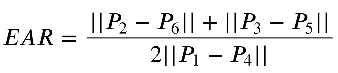
To detect whether the eyes are closed or not, we can use the Eye Aspect Ratio (EAR) formula:
The EAR formula returns a single scalar quantity that reflects the level of eye-opening.
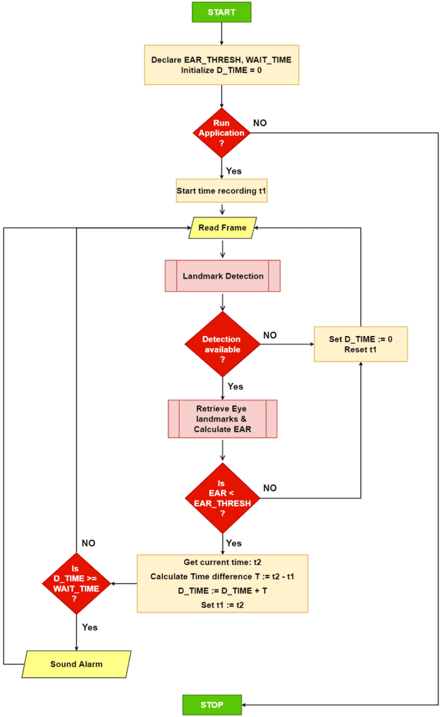
Our algorithm for the driver drowsiness detection system is as follows:
“We will track the EAR value across multiple consecutive frames. If the eyes have been closed for longer than some predetermined duration, we will set off the alarm.”
First, we declare two threshold values and a counter.
EAR_thresh:A threshold value to check whether the current EAR value is within range.
D_TIME: A counter variable to track the amount of time passed with current EAR < EAR_THRESH.
WAIT_TIME: To determine whether the amount of time passed with EAR < EAR_THRESH exceeds the permissible limit.
When the application starts, we record the current time (in seconds) in a variable t1 and read the incoming frame.
Next, we preprocess and pass the frame through Mediapipe’s Face Mesh solution pipeline.
We retrieve the relevant (Pi) eye landmarks if any landmark detections are available. Otherwise, reset t1and D_TIME (D_TIME is also reset over here to make the algorithm consistent).
If detections are available, calculate the average EAR valuefor both eyes using the retrieved eye landmarks.
If the current EAR < EAR_THRESH, add the difference between the current time t2 and t1 to D_TIME. Then reset t1 for the next frame as t2.
If the D_TIME >= WAIT_TIME, we sound the alarm or move on to the next frame.
Landmark Detection Using Mediapipe Face Mesh In Python
To learn more about Mediapipe, check out our introductory tutorial to Mediapipe, where we cover the different components of Mediapipe in great detail.
“Our ML pipeline consists of two real-time deep neural network models that work together: A detector that operates on the full image and computes face locations and a 3D face landmark model that operates on those locations and predicts the approximate 3D surface via regression. Having the face accurately cropped drastically reduces the need for common data augmentations like affine transformations consisting of rotations, translation, and scale changes. Instead, it allows the network to dedicate most of its capacity to coordinating prediction accuracy. In addition, in our pipeline, the crops can also be generated based on the face landmarks identified in the previous frame, and only when the landmark model could no longer identify face presence is the face detector invoked to relocalize the face.”
The red box indicates the cropped area as input to the landmark model, the red dots represent the 468 landmarks in 3D, and the green lines connecting landmarks illustrate the contours around the eyes, eyebrows, lips, and the entire face.
Mediapipe is a great tool that makes building applications very easy. You may also be interested in our other blog post where we use the Face Mesh solution to create Snapchat and Instagram filters using Mediapipe.
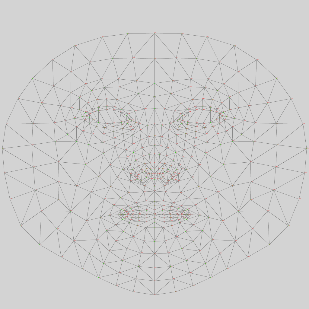
As stated above, the Face Mesh solution pipeline returns 468 landmark points on the face.
The below image shows the location of each of the points.
Note: The images captured by a camera are horizontally flipped. So, the landmarks (in the above image) in the eye (region) to your left are for the right eye and vice versa.
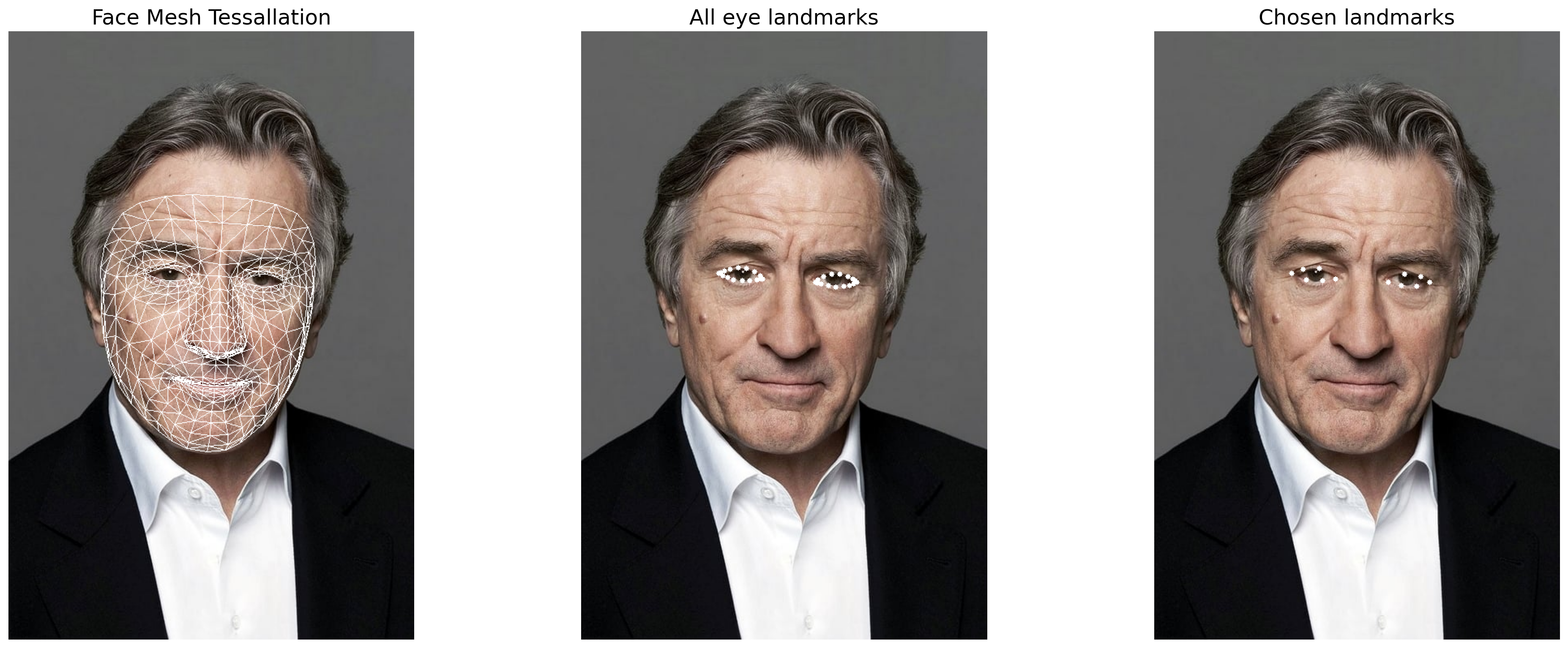
Since we are focusing on driver drowsiness detection, out of the 468 points, we only need landmark points belonging to the eye regions. The eye regions have 32 landmark points (16 points each).For calculating the EAR, we require only 12 points (6 for each eye).
With the above image as a reference, the 12 landmark points selected are as follows:
For the left eye: [362, 385, 387, 263, 373, 380]
For the right eye: [33, 160, 158, 133, 153, 144]
The chosen landmark points are in order: P1, P2, P3, P4, P5, P6
Please note that the above points are not coordinates. They denote an index position in the output list returned by the face mesh solution. To get the x, y (and z) coordinates, we must perform indexing on the returned list.
As mentioned in the description for the pipeline, the model first utilizes face detection along with a facial landmark detection model. For face detection, the pipeline uses the BlazeFace model, which has a very high inference speed.
Face detection is a very hot topic in the field of computer vision. To help our readers traverse the space easily, we’ve created a very in-depth guide to Face Detection post that compares the giants in this space.
Face Mesh Pipeline Demonstration
Let’s see how we can perform a simple inference using Face Mesh and plot the facial landmark points.
Download Code To easily follow along this tutorial, please download code by clicking on the button below. It's FREE!
The recommended way to initialize the Face Mesh graph object is using the “with” context manager. During initialization, we can also pass arguments such as:
static_image_mode: Whether to treat the input images as a batch of static and possibly unrelated images or a video stream.
max_num_faces: The maximum number of faces to detect.
refine_landmarks: Whether to further refine the landmark coordinates around the eyes and lips and other output landmarks around the irises.
min_detection_confidence: Minimum confidence value ([0.0, 1.0]) for face detection to be considered successful.
min_tracking_confidence: Minimum confidence value ([0.0, 1.0]) for the face landmarks to be considered tracked successfully.
# Running inference using static_image_mode
with mp_facemesh.FaceMesh(
    static_image_mode=True,         # Default=False
    max_num_faces=1,                # Default=1
    refine_landmarks=False,         # Default=False
    min_detection_confidence=0.5,   # Default=0.5
    min_tracking_confidence= 0.5,   # Default=0.5
) as face_mesh:

    results = face_mesh.process(image)

# Indicates whether any detections are available or not.
print(bool(results.multi_face_landmarks))
When you look at the pipeline arguments, an interesting parameter that pops up is min_tracking_confidence. As mentioned above, it’s to help with the continuous tracking of landmark points. So in between frames, instead of trying to continuously detect the faces, we can only track the movement of the detected face. As tracking algorithms are generally faster than detection algorithms, it further helps to improve the inference speed.
Object tracking is a fascinating domain in computer vision, and recently there have been great advancements in this field. If you want to learn more about the topic, do not worry, we’ve got you covered. We have a series of posts for you that will clearly explain how object tracking works?
Alright, at this point, we have confirmation that the pipeline has made some detections. The next task is to access the detected landmark points. We know that the pipeline can detect multiple faces and predict landmarks across all the detected faces. The results.multi_face_landmarks object is a list. Each index holds landmark detections for a face. The max length of this list depends on the max_num_facesparameter.
To get the first detected landmark point (of the only detected face), we have to use the .landmark attribute. You can think of it as a list of dictionaries. This attribute holds the normalized coordinates values of each detected landmark point.
Let’s see how to access the coordinates of the first landmark point of the first detected face.
x: 0.5087572336196899
y: 0.5726696848869324
z: -0.03815639764070511

X: 254.37861680984497
Y: 429.5022636651993
Z: -19.078198820352554

Total Length of '.landmark': 468
Let’s visualize the detected landmarks. We’ll plot the following:
All the detected landmarks using drawing_utils.
All eye landmarks.
Chosen eye landmarks.
For visualization, we’ll define a helper function.
def plot(
    *,
    img_dt,
    img_eye_lmks=None,
    img_eye_lmks_chosen=None,
    face_landmarks=None,
    ts_thickness=1,
    ts_circle_radius=2,
    lmk_circle_radius=3,
    name="1",
):
    # For plotting Face Tessellation
    image_drawing_tool = img_dt

     # For plotting all eye landmarks
    image_eye_lmks = img_dt.copy() if img_eye_lmks is None else img_eye_lmks

    # For plotting chosen eye landmarks
    img_eye_lmks_chosen = img_dt.copy() if img_eye_lmks_chosen is None else img_eye_lmks_chosen

    # Initializing drawing utilities for plotting face mesh tessellation
    connections_drawing_spec = mp_drawing.DrawingSpec(
        thickness=ts_thickness,
        circle_radius=ts_circle_radius,
        color=(255, 255, 255)
    )

    # Initialize a matplotlib figure.
    fig = plt.figure(figsize=(20, 15))
    fig.set_facecolor("white")

    # Draw landmarks on face using the drawing utilities.
    mp_drawing.draw_landmarks(
        image=image_drawing_tool,
        landmark_list=face_landmarks,
        connections=mp_facemesh.FACEMESH_TESSELATION,
        landmark_drawing_spec=None,
        connection_drawing_spec=connections_drawing_spec,
    )

    # Get the object which holds the x, y, and z coordinates for each landmark
    landmarks = face_landmarks.landmark

    # Iterate over all landmarks.
    # If the landmark_idx is present in either all_idxs or all_chosen_idxs,
    # get the denormalized coordinates and plot circles at those coordinates.

    for landmark_idx, landmark in enumerate(landmarks):
        if landmark_idx in all_idxs:
            pred_cord = denormalize_coordinates(landmark.x,
                                                landmark.y,
                                                imgW, imgH)
            cv2.circle(image_eye_lmks,
                       pred_cord,
                       lmk_circle_radius,
                       (255, 255, 255),
                       -1
                       )

        if landmark_idx in all_chosen_idxs:
            pred_cord = denormalize_coordinates(landmark.x,
                                                landmark.y,
                                                imgW, imgH)
            cv2.circle(img_eye_lmks_chosen,
                       pred_cord,
                       lmk_circle_radius,
                       (255, 255, 255),
                       -1
                       )

    # Plot post-processed images
    plt.subplot(1, 3, 1)
    plt.title("Face Mesh Tessellation", fontsize=18)
    plt.imshow(image_drawing_tool)
    plt.axis("off")

    plt.subplot(1, 3, 2)
    plt.title("All eye landmarks", fontsize=18)
    plt.imshow(image_eye_lmks)
    plt.axis("off")

    plt.subplot(1, 3, 3)
    plt.imshow(img_eye_lmks_chosen)
    plt.title("Chosen landmarks", fontsize=18)
    plt.axis("off")
    plt.show()
    plt.close()
    return
Now, to plot detections, we just have to iterate over the detections list.
# If detections are available.
if results.multi_face_landmarks:

    # Iterate over detections of each face. Here, we have max_num_faces=1,
    # So there will be at most 1 element in
    # the 'results.multi_face_landmarks' list
    # Only one iteration is performed.

    for face_id, face_landmarks in enumerate(results.multi_face_landmarks):
        _ = plot(img_dt=image.copy(), face_landmarks=face_landmarks)
The Eye Aspect Ratio (EAR) Technique
In the last section, we discussed the steps for point 2 of our solution. In this section, we will discuss point 3: The Eye Aspect Ratio formula introduced in the paper Real-Time Eye Blink Detection using Facial Landmarks.
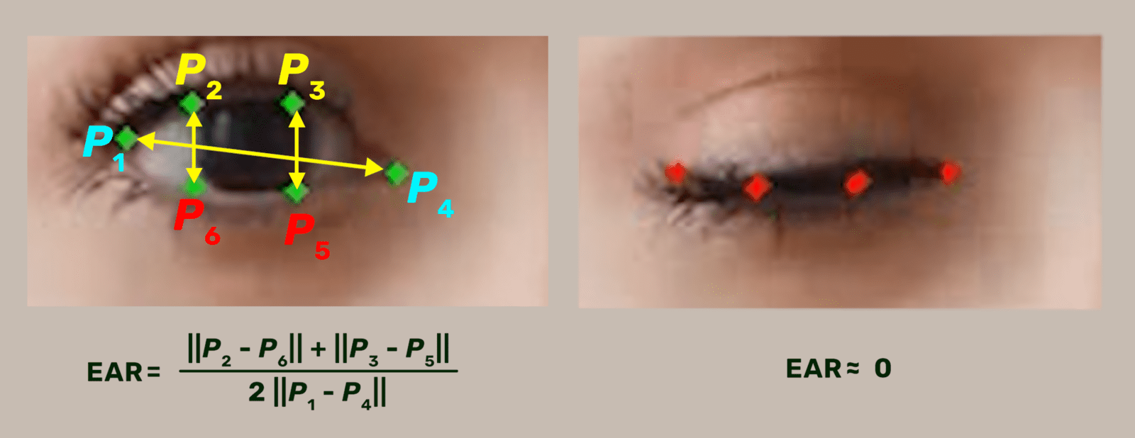
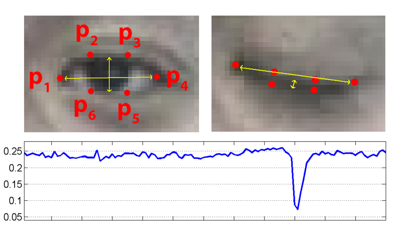
We will use Mediapipe’s Face Mesh solution to detect and retrieve the relevant landmarks in the eye region (points P1 – P6 in the below image).
After retrieving the relevant points, the Eye Aspect Ratio (EAR) is computed between the height and width of the eye.
The EAR is mostly constant when an eye is open and gets close to zero, while closing an eye is partially person, and head pose insensitive. The aspect ratio of the open eye has a small variance among individuals. It is fully invariant to a uniform scaling of the image and in-plane rotation of the face. Since eye blinking is performed by both eyes synchronously, the EAR of both eyes is averaged.
Top: Open and close eyes with landmarks Pi detected. Bottom: The eye aspect ratio EAR plotted for several frames of a video sequence. A single blink is present.
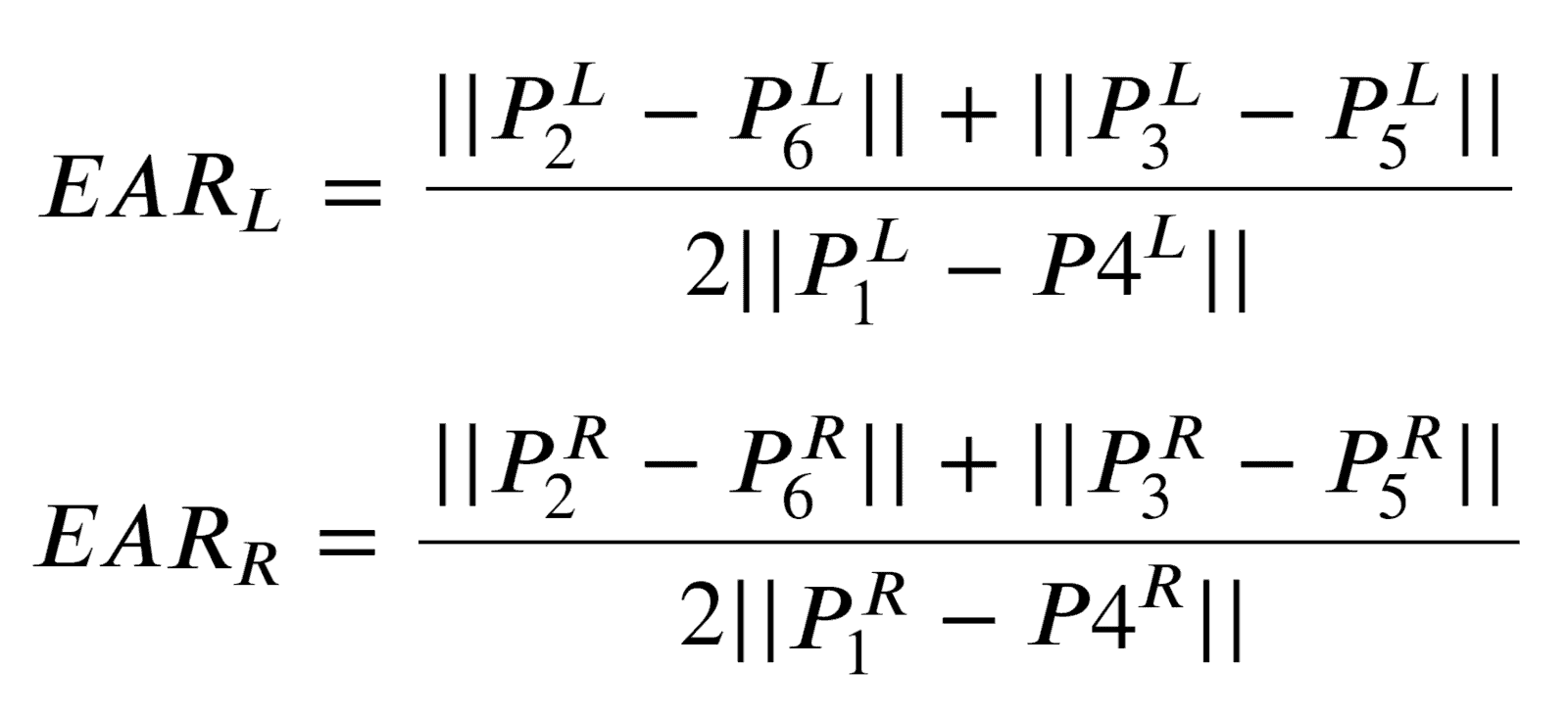
First, we have to calculate Eye Aspect Ratio for each eye:
The || (double pipe) indicates the L2 norm and is used to calculate the distance between two vectors.
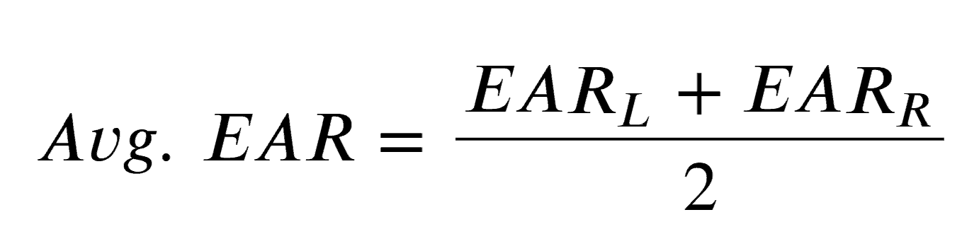
For calculating the final EAR value, the authors suggest averaging the two EAR values.
In general, the Avg. EAR value lies in range [0.0, 0.40]. The EAR value rapidly decreases during “eye closing” action.
Now that we are familiar with the EAR formula let’s define the three required functions: distance(…), get_ear(…), and calculate_avg_ear(…).
def distance(point_1, point_2):
    """Calculate l2-norm between two points"""
    dist = sum([(i - j) ** 2 for i, j in zip(point_1, point_2)]) ** 0.5
    return dist
The get_ear(…) function takes the .landmark attribute as a parameter. At each index position, we have a NormalizedLandmark object. This object holds the normalized x, y, and z coordinate values.
def get_ear(landmarks, refer_idxs, frame_width, frame_height):
    """
    Calculate Eye Aspect Ratio for one eye.

    Args:
        landmarks: (list) Detected landmarks list
        refer_idxs: (list) Index positions of the chosen landmarks
                            in order P1, P2, P3, P4, P5, P6
        frame_width: (int) Width of captured frame
        frame_height: (int) Height of captured frame

    Returns:
        ear: (float) Eye aspect ratio
    """
    try:
        # Compute the euclidean distance between the horizontal
        coords_points = []
        for i in refer_idxs:
            lm = landmarks[i]
            coord = denormalize_coordinates(lm.x, lm.y,
                                             frame_width, frame_height)
            coords_points.append(coord)

        # Eye landmark (x, y)-coordinates
        P2_P6 = distance(coords_points[1], coords_points[5])
        P3_P5 = distance(coords_points[2], coords_points[4])
        P1_P4 = distance(coords_points[0], coords_points[3])

        # Compute the eye aspect ratio
        ear = (P2_P6 + P3_P5) / (2.0 * P1_P4)

    except:
        ear = 0.0
        coords_points = None

    return ear, coords_points
Finally, the calculate_avg_ear(…) function is defined:
Let’s test the EAR formula. We will calculate the average EAR value for the previously used image and another image where the eyes are closed.
image_eyes_open  = cv2.imread("test-open-eyes.jpg")[:, :, ::-1]
image_eyes_close = cv2.imread("test-close-eyes.jpg")[:, :, ::-1]

for idx, image in enumerate([image_eyes_open, image_eyes_close]):

    image = np.ascontiguousarray(image)
    imgH, imgW, _ = image.shape

    # Creating a copy of the original image for plotting the EAR value
    custom_chosen_lmk_image = image.copy()

    # Running inference using static_image_mode
    with mp_facemesh.FaceMesh(refine_landmarks=True) as face_mesh:
        results = face_mesh.process(image).multi_face_landmarks

        # If detections are available.
        if results:
            for face_id, face_landmarks in enumerate(results):
                landmarks = face_landmarks.landmark
                EAR, _ = calculate_avg_ear(
                          landmarks,
                          chosen_left_eye_idxs,
                          chosen_right_eye_idxs,
                          imgW,
                          imgH
                      )

                # Print the EAR value on the custom_chosen_lmk_image.
                cv2.putText(custom_chosen_lmk_image,
                            f"EAR: {round(EAR, 2)}", (1, 24),
                            cv2.FONT_HERSHEY_COMPLEX,
                            0.9, (255, 255, 255), 2
                )

                plot(img_dt=image.copy(),
                     img_eye_lmks_chosen=custom_chosen_lmk_image,
                     face_landmarks=face_landmarks,
                     ts_thickness=1,
                     ts_circle_radius=3,
                     lmk_circle_radius=3
                )
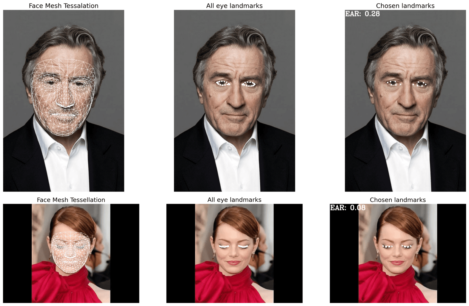
Result:
As you can observe, the EAR value when the eyes are open is 0.28 and (close to zero)0.08 when it’s close.
Driver Drowsiness Detection Code Walkthrough In Python
The previous sections covered all the required components for creating a driver drowsiness detection application. Now, we will start building our streamlit web app to make this application accessible to anyone using a web browser.
Straight off the bat, there’s an issue, streamlit doesn’t provide any component that can stream video from frontend to backend and back to frontend. It is not a problem if we only wish to use the application locally. There are workarounds where we can use OpenCV to connect to some IP cameras, but we won’t be using that approach here.
For our application, we will use an open-source streamlit component: streamlit-webrtc. It lets users handle and transmit real-time video/audio streams over a secure network with streamlit.
Let’s start.
First, we’ll create the drowsy_detection.pyscript (available in the download section). This script will contain all the functions and classes required for processing the input frame and tracking the state of different objects.
1) Importing necessary libraries and functions:
import cv2
import time
import numpy as np
import mediapipe as mp
from mediapipe.python.solutions.drawing_utils import _normalized_to_pixel_coordinates as denormalize_coordinates
2) Next, we’ll define the necessary functions. We have defined 3 functions, i.e., distance(…), get_ear(…) and calculate_avg_ear(…).
The new ones are:
get_mediapipe_app(…):To initialize the Mediapipe Face Mesh solution object.
plot_eye_landmarks(…):This function plots the detected (and the chosen) eye landmarks.
plot_text(…): This function is used to plot text on the video frames, such as the EAR value.
3) Next, we’ll define the VideoFrameHandlerclass. In this class, we’ll write the code for the algorithm discussed above. The two methods defined in this class are: __init__()andprocess(...).
Let’s go over them one by one.
class VideoFrameHandler:
    def __init__(self):
        """
        Initialize the necessary constants, mediapipe app
        and tracker variables
        """
        # Left and right eye chosen landmarks.
        self.eye_idxs = {
            "left": [362, 385, 387, 263, 373, 380],
            "right": [33, 160, 158, 133, 153, 144],
        }

        # Used for coloring landmark points.
        # Its value depends on the current EAR value.
        self.RED = (0, 0, 255)  # BGR
        self.GREEN = (0, 255, 0)  # BGR

        # Initializing Mediapipe FaceMesh solution pipeline
        self.facemesh_model = get_mediapipe_app()

        # For tracking counters and sharing states in and out of callbacks.
        self.state_tracker = {
            "start_time": time.perf_counter(),
            "DROWSY_TIME": 0.0,  # Holds time passed with EAR < EAR_THRESH
            "COLOR": self.GREEN,
            "play_alarm": False,
        }

        self.EAR_txt_pos = (10, 30)
First, we create a self.eye_idxsdictionary. This dictionary holds our chosen left and right eye landmark index positions.
The two color variables, self.RED and self.GREEN, are used to color landmark points, EAR value, and the DROWSY_TIME counter variable depending on the condition.
Next, we initialize the Mediapipe Face Mesh solution.
Finally, we define the self.state_tracker dictionary. This dictionary holds all the variables whose values keep changing. Specifically, it holds the start_time and DROWSY_TIME variables, crucial to our algorithm.
Finally, we have to define the coordinate position where we will print the current average EAR value on the frame.
Next, let’s go over the process(…) method:
def process(self, frame: np.array, thresholds: dict):
        """
        This function is used to implement our Drowsy detection algorithm.

        Args:
            frame: (np.array) Input frame matrix.
            thresholds: (dict) Contains the two threshold values
                               WAIT_TIME and EAR_THRESH.

        Returns:
            The processed frame and a boolean flag to
            indicate if the alarm should be played or not.
        """

        # To improve performance,
        # mark the frame as not writeable to pass by reference.
        frame.flags.writeable = False
        frame_h, frame_w, _ = frame.shape
        DROWSY_TIME_txt_pos = (10, int(frame_h // 2 * 1.7))
        ALM_txt_pos = (10, int(frame_h // 2 * 1.85))

        results = self.facemesh_model.process(frame)

        if results.multi_face_landmarks:
            landmarks = results.multi_face_landmarks[0].landmark
            EAR, coordinates = calculate_avg_ear(landmarks,
                                                 self.eye_idxs["left"],
                                                 self.eye_idxs["right"],
                                                 frame_w,
                                                 frame_h
                                                 )
            frame = plot_eye_landmarks(frame,
                                       coordinates[0],
                                       coordinates[1],
                                       self.state_tracker["COLOR"]
                                       )

            if EAR < thresholds["EAR_THRESH"]:

                # Increase DROWSY_TIME to track the time period with
                # EAR less than the threshold
                # and reset the start_time for the next iteration.
                end_time = time.perf_counter()

                self.state_tracker["DROWSY_TIME"] += end_time - self.state_tracker["start_time"]
                self.state_tracker["start_time"] = end_time
                self.state_tracker["COLOR"] = self.RED

                if self.state_tracker["DROWSY_TIME"] >= thresholds["WAIT_TIME"]:
                    self.state_tracker["play_alarm"] = True
                    plot_text(frame, "WAKE UP! WAKE UP",
                              ALM_txt_pos, self.state_tracker["COLOR"])

            else:
                self.state_tracker["start_time"] = time.perf_counter()
                self.state_tracker["DROWSY_TIME"] = 0.0
                self.state_tracker["COLOR"] = self.GREEN
                self.state_tracker["play_alarm"] = False

            EAR_txt = f"EAR: {round(EAR, 2)}"
            DROWSY_TIME_txt = f"DROWSY: {round(self.state_tracker['DROWSY_TIME'], 3)} Secs"
            plot_text(frame, EAR_txt,
                      self.EAR_txt_pos, self.state_tracker["COLOR"])
            plot_text(frame, DROWSY_TIME_txt,
                      DROWSY_TIME_txt_pos, self.state_tracker["COLOR"])

        else:
            self.state_tracker["start_time"] = time.perf_counter()
            self.state_tracker["DROWSY_TIME"] = 0.0
            self.state_tracker["COLOR"] = self.GREEN
            self.state_tracker["play_alarm"] = False

            # Flip the frame horizontally for a selfie-view display.
            frame = cv2.flip(frame, 1)

        return frame, self.state_tracker["play_alarm"]
Here,
We start by setting the .writeable flag on the frame NumPy array to False. This helps to improve performance. So instead of sending a copy of the frameto each function, we send a reference to the frame.
Next, we initialize some text position constants considering the current frame dimensions.
The input frame passed to this method will be in RGB format. This is the only preprocessing required. The Mediapipe modeltakes thisframe as input. The output is collected in the resultsobject.
From this point on, the code reflects the algorithm flowchart we have discussed above.
The 1st if-check is to determine if any detections are available or not. If True, the calculate_avg_ear(…) function calculates the average EAR value. This function also returns the current denormalized coordinates position for the chosen landmarks. The plot_eye_landmarks(…) plots these denormalized coordinates.
Next in line is the 2nd if-check to determine whether the current EAR < EAR_THRESH. If True, we record the difference between the current_time (end_time) and start_time. The DROWSY_TIMEcounter value is incremented based on this difference. Then, we reset start_time to end_time. It helps by tracking the time between the current and next frame (if the EAR is still less than EAR_THRESH).
The 3rd if-check is to determine whether the DROWSY_TIME >= WAIT_TIME. The WAIT_TIME threshold holds the value of the allowed amount of time with eyes closed.
If the 3rd condition is True, we set the state of the play_alarm boolean flag to True.
If the 1st and 2nd conditions are False, reset the state variables. The state of the COLOR variable also changes based on the above conditions. The text color for printing EAR and DROWSY_TIME onto the frame depends on the COLOR state.
Finally, we return the processed frame and the value of the play_alarmstate variable.
This concludes the drowsy_detection.py script.
Next, we will create the streamlit_app.pyscript. This file contains the UI components of our web app, such as the slider components (for adjusting thresholds) and buttons used in our application. It also includes the code related to the streamlit-webrtc library.
(This script and the rest of the assets are available in the download code section.)
import os
import av
import threading
import streamlit as st
from streamlit_webrtc import VideoHTMLAttributes, webrtc_streamer

from audio_handling import AudioFrameHandler
from drowsy_detection import VideoFrameHandler

# Define the audio file to use.
alarm_file_path = os.path.join("audio", "wake_up.wav")

# Streamlit Components
st.set_page_config(
    page_title="Drowsiness Detection | LearnOpenCV",
    page_icon="https://learnopencv.com/wp-content/uploads/2017/12/favicon.png",
    layout="centered",
    initial_sidebar_state="expanded",
    menu_items={
        "About": "### Visit www.learnopencv.com for more exciting tutorials!!!",
    },
)

st.title("Drowsiness Detection!")

col1, col2 = st.columns(spec=[1, 1])

with col1:
    # Lowest valid value of Eye Aspect Ratio. Ideal values [0.15, 0.2].
    EAR_THRESH = st.slider("Eye Aspect Ratio threshold:", 0.0, 0.4, 0.18, 0.01)

with col2:
    # The amount of time (in seconds) to wait before sounding the alarm.
    WAIT_TIME = st.slider("Seconds to wait before sounding alarm:", 0.0, 5.0, 1.0, 0.25)

thresholds = {
    "EAR_THRESH": EAR_THRESH,
    "WAIT_TIME": WAIT_TIME,
}

# For streamlit-webrtc
video_handler = VideoFrameHandler()
audio_handler = AudioFrameHandler(sound_file_path=alarm_file_path)

# For thread-safe access & to prevent race-condition.
lock = threading.Lock()

shared_state = {"play_alarm": False}

def video_frame_callback(frame: av.VideoFrame):
    frame = frame.to_ndarray(format="bgr24")  # Decode and convert frame to RGB

    frame, play_alarm = video_handler.process(frame, thresholds)  # Process frame
    with lock:
        shared_state["play_alarm"] = play_alarm  # Update shared state

    # Encode and return BGR frame
    return av.VideoFrame.from_ndarray(frame, format="bgr24")

def audio_frame_callback(frame: av.AudioFrame):
    with lock:  # access the current “play_alarm” state
        play_alarm = shared_state["play_alarm"]

    new_frame: av.AudioFrame = audio_handler.process(frame,
                                                     play_sound=play_alarm)
    return new_frame

ctx = webrtc_streamer(
    key="driver-drowsiness-detection",
    video_frame_callback=video_frame_callback,
    audio_frame_callback=audio_frame_callback,
    rtc_configuration={"iceServers": [{"urls": ["stun:stun.l.google.com:19302"]}]},
    media_stream_constraints={"video": {"width": True, "audio": True},
    video_html_attrs=VideoHTMLAttributes(autoPlay=True, controls=False, muted=False),
)
We start by importing the necessary libraries and the two special classes we have created, VideoFrameHandler and AudioFrameHandler. I’ll discuss the functionality of the AudioFrameHandler class shortly.
Next, we declare the streamlit-basedcomponents, such as page configs, title, and the two sliders (EAR_THESHand WAIT_TIME). We will pass these values to the VideoHandler’s process(…) method.
Next, we initialize the two custom class instances: video_handlerand audio_handler.
Then we initialize the thread lock and a shared_state dictionary object. The dictionary object holds just one key-value pair, i.e., play_alarmboolean flag. Its value depends on the play_alarmboolean returned by the .process(…) method of VideoFrameHandler class.
The (mutable) shared_state dictionary is used to help pass state information between the two functions: video_frame_callback and audio_frame_callback.
The video_frame_callback function is defined for processing the input video frames. It receives one frame at a time from the front end.
Similarly, the audio_frame_callbackfunction is used for processing and returning custom audio frames such as an alarm sound.
Finally, we create the streamlit-webrtc component webrtc-streamer. It will handle the secure transmission of data frames between the user and server.
And that concludes the streamlit_app.py script.
Note: The video_frame_callbackreceives a VideoFrameobject (of some dimension), and the audio_frame_callbackreceivesan AudioFrame object (of some length). There is one limitation to streamlit-webrtc. The user needs to provide permission for the webcam and the microphone for the application to work. As of writing this post, there’s no way to only receive and return video frames with occasional audio data (when a condition is met).
The only remaining script is the audio_handling.py file, which contains the AudioFrameHandlerclass. Here, we won’t be going over the code, but we’ll provide the gist of the functionality performed by this class. We’ll discuss how each audio frame is processed.
In the audio_frame_callbackfunction we defined above, at each timestamp, we receive an audio frame of some length, shape, frame_rate, channels, etc.
For, e.g., let’s say the input audio frame is 20 ms long. Now, there is a problem because our alarm/sound file can be of any duration long. And we cannot send the entire alarm sound in one go. If we compress and send it, the audio will just be a short burst of noise.
The solution is to chop up the alarm sound file into sizes of 20ms long segments. Then, if the play_alarm flag is True, keep returning the chopped alarm file segments one by one until we send the last segment.
One way to look at this solution is: When speaking, we don’t cram everything we want to say in (say) 20 ms, but it’s spread across some time (>20ms). In each instance, we deliver only a portion of our entire sentence. The complete sentence comprises all these minute components that have been spread over time and linked together repeatedly.
In the audio_frame_callbackfunction, the .process(...) method is called each time with a different input audio segment.
The properties of this audio segment can differ between different connections and browsers. The .prepare_audio(…) function is called on the first input audio frame to handle this issue.
Depending on the properties of the input audio frame, the alarm sound file is processed and chopped into segments accordingly.
Then, depending on the play_soundboolean flag, we either return chopped alarm sound file segments or change the amplitude (generally, loudness) of the input audio segment by -100. It dampens the entire input sound wave and provides the silence effect.
That concludes the final audio_handling.py script.
In this post, our goal was to create a simple and helpful Driver Drowsiness Detection application using Mediapipe in Python. We began by defining the problem statement and stating a relevant use case. We then proposed an effective, fast, and easy-to-implement solution in python. We leveraged Mediapipe’s Face Mesh pipeline and the Eye aspect ratio formula for the solution. The web app’s UI component is built using Streamlit and streamlit-webrtc. Finally, we demonstrate our web app deployed on cloud service.
This is just one possible solution. Another possible solution is to use some algorithm (maybe the same Face Mesh pipeline), extract the eye regions from the frame, and pass them through a deep learning-based classifier. We will demonstrate more of such applications in our future articles. As of now, it’s up to the reader to explore and master the above options.
If you liked this article and would like to download code (C++ and Python) and example images used in this post, please click here. Alternately, sign up to receive a free Computer Vision Resource Guide. In our newsletter, we share OpenCV tutorials and examples written in C++/Python, and Computer Vision and Machine Learning algorithms and news.
This course is available for FREE only till 22nd Nov.
FREE Python Course
We have designed this Python course in collaboration with OpenCV.org for you to build a strong foundation in the essential elements of Python, Jupyter, NumPy and Matplotlib.
We hate SPAM and promise to keep your email address safe.
FREE OpenCV Crash Course
We have designed this FREE crash course in collaboration with OpenCV.org to help you take your first steps into the fascinating world of Artificial Intelligence and Computer Vision. The course will be delivered straight into your mailbox.
We hate SPAM and promise to keep your email address safe.
Get Started with OpenCV
FREE OpenCV Crash Course
Getting Started Guides
Installation Packages
C++ And Python Examples
Newsletter Insights
We hate SPAM and promise to keep your email address safe.
Subscribe to receive the download link, receive updates, and be notified of bug fixes
Which email should I send you the download link?
We hate SPAM and promise to keep your email address safe.
Subscribe To Receive
FREE OpenCV Crash Course
Getting Started Guides
Installation Packages
C++ And Python Examples
Newsletter Insights
We hate SPAM and promise to keep your email address safe.
We hate SPAM and promise to keep your email address safe.
Subscribe Now
About LearnOpenCV
Empowering innovation through education, LearnOpenCV provides in-depth tutorials, code, and guides in AI, Computer Vision, and Deep Learning. Led by Dr. Satya Mallick, we're dedicated to nurturing a community keen on technology breakthroughs.