Stanford ML Group, led by Andrew Ng, works on important problems in areas such as healthcare and climate change, using AI.

Last year they released a knee MRI dataset consisting of 1,370 knee MRI exams performed at Stanford University Medical Center. Subsequently, the MRNet challenge was also announced.

Source: Stanford ML Group

For those wishing to enter the field for AI in medical imaging, we believe that this dataset is just the right one for you. The challenge problem statement is neither too easy nor too difficult. The uniqueness and subtle complexities of the dataset will surely help you explore new thought processes and grow.

And don’t forget, we are here to guide you on how to approach the problem at hand.

So let’s dive right in!!

This post will be covering the topics

Exploring the MRNet dataset
The problem at hand (The Challenge)
Our approach
Model Architecture
Results
An alternative approach

Deep Learning to Classify MRIs

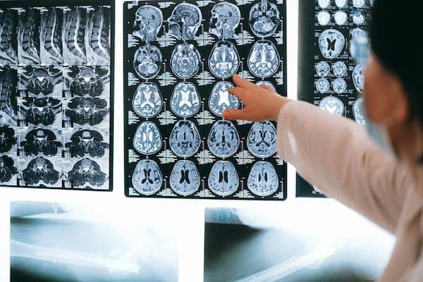
Interpretation of any kind of MRI is time-intensive and subject to diagnostic error and variability. Therefore automated system for interpreting this type of image data could prioritize high-risk patients and assist clinicians in making diagnoses.

Have a look at this article if you are interested in knowing more about using deep learning with MRI scans

Moreover, a system that produces less false positives than a radiologist is very advantageous because it eliminates the risk of performing unnecessary invasive surgeries.

We think that deep learning will soon help radiologists make faster and more accurate diagnoses.

The MRNet Dataset

The MRNet dataset consists of 1,370 knee MRI exams performed at Stanford University Medical Center. The dataset contains abnormal exams, with ACL tears and meniscal tears.

Labels were obtained through manual extraction from clinical reports. The dataset accompanies the publication of the MRNet work here.

I. Explaining the dataset

The dataset contains MRIs of different people in .npy file format. Each MRI consists of multiple images (or slices). The number of slices has to do with the way MRI is taken of a particular body part. What happens is we pick a cross-section plane, and then move that plane across the body part, taking snapshots at different instances. So in this way, an image consists of different slices.

MRNet consists of images with variable slices across three planes, namely axial, coronal, and sagittal.

So an image will have dimensions [slices, 256, 256].

There are three folders with the same name as the three planes discussed above, and each image in each of these three folders is a collection of snapshots at different intervals.

The labels are present in the correspondingly named .csv file. Each image in each plane has a label of 0 or 1, where 0 means that the MRI showed does not have the disease and 1 means that MRI shown has that disease.

II. Uniqueness of Dataset and Splits

The exams have been split into three sets

Training set (1,130 exams, 1,088 patients)
Validation set (called tuning set in the paper) (120 exams, 111 patients)
Hidden test set (called the validation set in the paper) (120 exams, 113 patients).

To form the validation and tuning sets, stratified random sampling was used to ensure that at least 50 positive examples of each label (abnormal, ACL tear, and meniscal tear) were present in each set. All exams from each patient were put in the same split.

To evaluate your model on the hidden test set, you have to submit your model on CodaLab (more details are present on the challenge website).

III. Visualizing the data

The dataset contains images as shown below

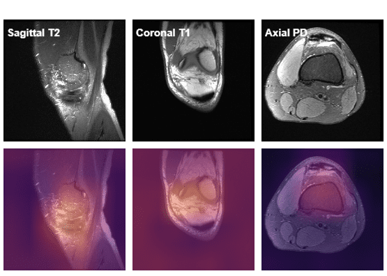
There is some awesome work done on visualizing this dataset by Ahmed Besbes. Do check out his work here.

The MRNet Challenge

We were asked to do binary classification for each disease separately. Instead of predicting the class, we were asked to predict the probability that the MRI is of positive class. We then calculate area under ROC curve for predictions for each disease and then take average to report the average AUC as the final score.

Obstacles in our Approach

One thing we noticed is that slices are significantly different from one plane to another. Not just this, the number of slices are also different for the same MRI scan across different planes, for eg. an image across axial plane may have dimensions [25, 256, 256], whereas the same MRI has dimension [29, 256, 256] in coronal plane.

Also within the same plane, images may differ a lot since they were taken at different timestamps, eg. at one time the plane would have been completely inside the knee, whereas some other time it would have just grazed the knee from above, thereby resulting in very different images within a single plane too.

Due to the variable slices problem, multiple MRI scan couldn’t be put in a single batch, so we used a batch of one patient only.

Our Approach

Initially our plan was to train 9 CNN models – one for each disease across each plane.

But then later we decided – why not combine information across three planes to make a prediction for each disease? So we finalised to make a model for each disease that accepts images from all three planes and uses them to predict whether the patient has that particular disease or not.

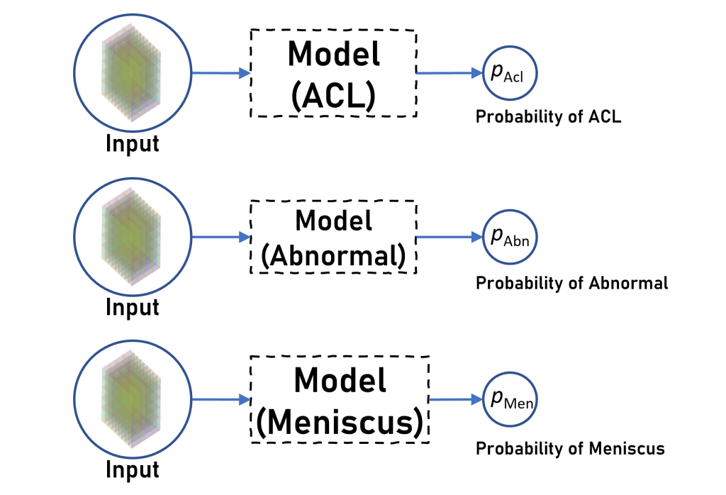
So effectively we are now training 3 CNN models (one for each disease) which is quite less than the 9 CNN models that we were planning on initially.

Download Code To easily follow along this tutorial, please download code by clicking on the button below. It's FREE!

Click here to download the source code to this post

Model Architecture

class MRnet(nn.Module):
    """MRnet uses pretrained resnet50 as a backbone to extract features
    """
     
    def __init__(self):
        """This function will be used to initialize the 
        MRnet instance."""
        # Initialize nn.Module instance
        super(MRnet,self).__init__()
 
        # Initialize three backbones for three axis
        # All the three axes will use pretrained AlexNet model
        # The models will be used for extracting features from
        # the input images
        self.axial = models.alexnet(pretrained=True).features
        self.coronal = models.alexnet(pretrained=True).features
        self.saggital = models.alexnet(pretrained=True).features
         
        # Initialize 2D Adaptive Average Pooling layers
        # The pooling layers will reduce the size of
        # feature maps extracted from the previous axes
        self.pool_axial = nn.AdaptiveAvgPool2d(1)
        self.pool_coronal = nn.AdaptiveAvgPool2d(1)
        self.pool_saggital = nn.AdaptiveAvgPool2d(1)
         
        # Initialize a sequential neural network with
        # a single fully connected linear layer
        # The network will output the probability of
        # having a particular disease
        self.fc = nn.Sequential(
            nn.Linear(in_features=3*256,out_features=1)
        )

The model is surprisingly simple, we make a class MRNet that inherits from the torch.nn.Module class.

In the __init__ method, we define three pretrained alexnet models for each of the three planes namely axial, sagittal and coronal. We use this backbone networks as a feature extractor, that is why we just use the .features of the alexnet and ignore the classification head of the alexnet.

Then a AdaptiveAveragePool layer reduces the size of the feature image that we extracted from alexnet.features backbone.

Finally we define a fully connected layer fc with input dimension size 3 x 256, and output dimension as 1 (a single neuron) to predict the probability of the patient having a particular disease.

Backbone Network Used

As discussed above, we used AlexNet network pretrained network as a feature extractor. Please note – it was just a personal preference to use AlexNet, we could have used ResNet as well for backbone.

Input

So the input we expect are three images in a list i.e. [image1, image2, image3] where each image is a stack of slices across each plane, i.e image1 is stack of slices across the axial plane.

If we look at image1, its dimension is of the form [1, slices, 3, 224, 224], the extra 1 in the beginning of the image1 dimension is due to the Data Loader adding a extra dimension to it.

Output

We output a single logit denoting the probability of the patient having a particular disease. We don’t take sigmoid in the forward method as during calculation of the loss, BCELoss has torch.sigmoid built in.

Forward Method

def forward(self,x):
        """ Input is given in the form of `[image1, image2, image3]` where
        `image1 = [1, slices, 3, 224, 224]`. Note that `1` is due to the 
        dataloader assigning it a single batch. 
        """
 
        # squeeze the first dimension as there
        # is only one patient in each batch
        images = [torch.squeeze(img, dim=0) for img in x]
         
        # Extract features across each of the three plane
        # using the three pre-trained AlexNet models defined earlier
        image1 = self.axial(images[0])
        image2 = self.coronal(images[1])
        image3 = self.saggital(images[2])
 
        # Convert the image dimesnsions from [slices, 256, 1, 1] to
        # [slices,256]
        image1 = self.pool_axial(image1).view(image1.size(0), -1)
        image2 = self.pool_coronal(image2).view(image2.size(0), -1)
        image3 = self.pool_saggital(image3).view(image3.size(0), -1)
 
        # Find maximum value across slices
        # This will reduce the dimensions of image to [1,256]
        # This is done in order to keep only the most prevalent
        # features for each slice
        image1 = torch.max(image1,dim=0,keepdim=True)[0]
        image2 = torch.max(image2,dim=0,keepdim=True)[0]
        image3 = torch.max(image3,dim=0,keepdim=True)[0]
 
        # Stack the 3 images together to create the output
        # of size [1, 256*3]
        output = torch.cat([image1,image2,image3], dim=1)
 
        # Feed the output to the sequential network created earlier
        # The network will return a probability of having a specific
        # disease
        output = self.fc(output)
        return output

We first squeeze the first dimension of each image as it is redundant. So the current dimension becomes of each image[i] becomes[slices, 3, 224, 224]

Then we pass each image through the AlexNet backbones to extract features across each plane. So the dimension of each image currently is [slices, 256, 7, 7]

We then take a Average Pool, which converts the dimension of each image to [slices, 256, 1, 1], which we then convert it to [slices, 256] using the .view() function.

Now we pick the maximum value across slices, so the dimension of each image now becomes [1, 256]. This step is important in order to handle the variable size of slices in each plane, we only most prevalent features in each slice.

We then stack these three images of three planes together to form a final tensor of size [1, 3 * 256] or [1, 768].

We then pass it to the fully connected layer fc that results in the output of size [1, 1].

Data Loader

We created a class MRData that inherits and implemented two functions namely __len__ and __getitem__ as required by torch.utils.data.DataLoader.

Nothing too complex in __init__ method as well, we just read the required .csv files that contain the filenames for MRIs and their respective labels.

We also calculate the weight for the +ve class that we pass to the loss function as will be discussed below in more detail.

class MRData():
    """This class used to load MRnet dataset from `./images` dir
    """
 
    def __init__(self,task = 'acl', train = True, transform = None, weights = None):
        """Initialize the dataset
        Args:
            plane : along which plane to load the data
            task : for which task to load the labels
            train : whether to load the train or val data
            transform : which transforms to apply
            weights (Tensor) : Give wieghted loss to postive class eg. `weights=torch.tensor([2.223])`
        """
        # Define the three planes to use
        self.planes=['axial', 'coronal', 'sagittal']
        # Initialize the records as None
        self.records = None
        # an empty dictionary
        self.image_path={}
         
        # If we are in training loop
        if train:
            # Read data about patient records
            self.records = pd.read_csv('./images/train-{}.csv'.format(task),header=None, names=['id', 'label'])
 
            for plane in self.planes:
                # For each plane, specify the image path
                self.image_path[plane] = './images/train/{}/'.format(plane)
        else:
            # If we are in testing loop
            # don't use any transformation
            transform = None
            # Read testing/validation data (patients records)
            self.records = pd.read_csv('./images/valid-{}.csv'.format(task),header=None, names=['id', 'label'])
             
            for plane in self.planes:
                # Read path of images for each plane
                self.image_path[plane] = './images/valid/{}/'.format(plane)
 
        # Initialize the transformation to apply on images
        self.transform = transform 
 
        # Append 0s to the patient record id
        self.records['id'] = self.records['id'].map(
            lambda i: '0' * (4 - len(str(i))) + str(i))
        # empty dictionary
        self.paths={}
        for plane in self.planes:
            # Get paths of numpy data files for each plane
            self.paths[plane] = [self.image_path[plane] + filename +
                          '.npy' for filename in self.records['id'].tolist()]
 
        # Convert labels from Pandas Series to a list
        self.labels = self.records['label'].tolist()
 
        # Total positive cases
        pos = sum(self.labels)
        # Total negative cases
        neg = len(self.labels) - pos
 
        # Find the wieghts of pos and neg classes
        if weights:
            self.weights = torch.FloatTensor(weights)
        else:
            self.weights = torch.FloatTensor([neg / pos])
         
        print('Number of -ve samples : ', neg)
        print('Number of +ve samples : ', pos)
        print('Weights for loss is : ', self.weights)
 
    def __len__(self):
        """Return the total number of images in the dataset."""
        return len(self.records)
 
    def __getitem__(self, index):
        """
        Returns `(images,labels)` pair
        where image is a list [imgsPlane1,imgsPlane2,imgsPlane3]
        and labels is a list [gt,gt,gt]
        """
        img_raw = {}
         
        for plane in self.planes:
            # Load raw image data for each plane
            img_raw[plane] = np.load(self.paths[plane][index])
            # Resize the image loaded in the previous step
            img_raw[plane] = self._resize_image(img_raw[plane])
             
        label = self.labels[index]
        # Convert label to 0 and 1
        if label == 1:
            label = torch.FloatTensor([1])
        elif label == 0:
            label = torch.FloatTensor([0])
 
        # Return a list of three images for three planes and the label of the record
        return [img_raw[plane] for plane in self.planes], label
 
    def _resize_image(self, image):
        """Resize the image to `(3,224,224)` and apply 
        transforms if possible.
        """
        # Resize the image
        # Calculate extra padding present in the image
        # which needs to be removed
        pad = int((image.shape[2] - INPUT_DIM)/2)
        # This is equivalent to center cropping the image
        image = image[:,pad:-pad,pad:-pad]
        # Normalize the image by subtracting it by mean and dividing by standard
        # deviation
        image = (image-np.min(image))/(np.max(image)-np.min(image))*MAX_PIXEL_VAL
        image = (image - MEAN) / STDDEV
         
        # If the transformation is not None
        if self.transform:
            # Transform the image based on the specified transformation
            image = self.transform(image)
        else:
            # Else, just stack the image with itself in order to match the required
            # dimensions
            image = np.stack((image,)*3, axis=1)
        # Convert the image to a FloatTensor and return it
        image = torch.FloatTensor(image)
        return image

One thing to note is that before returning we have to resize the images to [224, 224] from [256, 256] across each slice. Also since alexnet backbone accepts images having three color channels, we could just stack the single image three times to overcome this issue however there is a better way.

Augmentations to the rescue!!

Instead of stacking the same image thrice, why not apply different augmentations to an image and then stack the resulting images together to overcome the 3 color channel problem. In this way, we fix the problem, but also add more diversity to our dataset that will help our model to generalize better.

def load_data(task : str):
 
    # Define the Augmentation here only
    augments = Compose([
        # Convert the image to Tensor
        transforms.Lambda(lambda x: torch.Tensor(x)),
        # Randomly rotate the image with an angle
        # between -25 degrees to 25 degrees
        RandomRotate(25),
        # Randomly translate the image by 11% of 
        # image height and width
        RandomTranslate([0.11, 0.11]),
        # Randomly flip the image
        RandomFlip(),
        # Change the order of image channels
        transforms.Lambda(lambda x: x.repeat(3, 1, 1, 1).permute(1, 0, 2, 3)),
    ])
 
    print('Loading Train Dataset of {} task...'.format(task))
    # Load training dataset
    train_data = MRData(task, train=True, transform=augments)
    train_loader = data.DataLoader(
        train_data, batch_size=1, num_workers=11, shuffle=True
    )
 
    print('Loading Validation Dataset of {} task...'.format(task))
    # Load validation dataset
    val_data = MRData(task, train=False)
    val_loader = data.DataLoader(
        val_data, batch_size=1, num_workers=11, shuffle=False
    )
 
    return train_loader, val_loader, train_data.weights, val_data.weights

Some image transformations we apply are randomly rotating the image 25 degrees to left or right. Also, we add a little bit of translational shift as well. We also apply some random flipping of the image upside down.

We use the load_data function as shown above to return iterators to train dataset and validation dataset.

Loss Function Used

Since this is a binary classification problem, Binary Cross Entropy Loss is the way to go. However, since our dataset had some class imbalances, we went for a weighted BCE Loss.

We use torch.nn.BCEWithLogitsLoss to calculate the loss. This calls the torch.sigmoid internally which is numerically more stable. That is why it accepts raw logits from the model, hence the name.

It also accepts the parameter, pos_weight which is used to positively weight a class while calculating loss. We assigned this parameter as no. of -ve samples/ no. of +ve samples.

A thing to note here is that we don’t need a negative weight here as the loss method just gives it a weight of 1.0.

Learning Rate (LR) strategy

We use a strategy that reduces the learning rate by a factor of 3.0 whenever the Validation Loss plateaus for 3 consecutive epochs, with a threshold of 1e-4.

Evaluation Metric Used

We use the Area under the the ROC curve to judge the performance of the model for each disease. We then average these AUCs for all three diseases to get a final performance score of the model.

If you don’t know what AUC and ROC means, I recommend that you check this article out, it explains these concepts quite lucidly

Training Loop

Below is the code for train loop for one epoch.

def _train_model(model, train_loader, epoch, num_epochs, optimizer, criterion, writer, current_lr, log_every=100):
     
    # Set to train mode
    model.train()
 
    # Initialize the predicted probabilities
    y_probs = []
    # Initialize the groundtruth labels
    y_gt = []
    # Initialize the loss between the groundtruth label
    # and the predicted probability
    losses = []
 
    # Iterate over the training dataset
    for i, (images, label) in enumerate(train_loader):
        # Reset the gradient by zeroing it
        optimizer.zero_grad()
         
        # If GPU is available, transfer the images and label
        # to the GPU
        if torch.cuda.is_available():
            images = [image.cuda() for image in images]
            label = label.cuda()
 
        # Obtain the prediction using the model
        output = model(images)
 
        # Evaluate the loss by comparing the prediction
        # and groundtruth label
        loss = criterion(output, label)
        # Perform a backward propagation
        loss.backward()
        # Modify the weights based on the error gradient
        optimizer.step()
 
        # Add current loss to the list of losses
        loss_value = loss.item()
        losses.append(loss_value)
 
        # Find probabilities from output using sigmoid function
        probas = torch.sigmoid(output)
 
        # Add current groundtruth label to the list of groundtruths
        y_gt.append(int(label.item()))
        # Add current probabilities to the list of probabilities
        y_probs.append(probas.item())
 
        try:
            # Try finding the area under ROC curve
            auc = metrics.roc_auc_score(y_gt, y_probs)
        except:
            # Use default value of area under ROC curve as 0.5
            auc = 0.5
         
        # Add information to the writer about training loss and Area under ROC curve
        writer.add_scalar('Train/Loss', loss_value,
                          epoch * len(train_loader) + i)
        writer.add_scalar('Train/AUC', auc, epoch * len(train_loader) + i)
 
        if (i % log_every == 0) & (i > 0):
            # Display the information about average training loss and area under ROC curve
            print('''[Epoch: {0} / {1} | Batch : {2} / {3} ]| Avg Train Loss {4} | Train AUC : {5} | lr : {6}'''.
                  format(
                      epoch + 1,
                      num_epochs,
                      i,
                      len(train_loader),
                      np.round(np.mean(losses), 4),
                      np.round(auc, 4),
                      current_lr
                  )
                  )
    # Add information to the writer about total epochs and Area under ROC curve
    writer.add_scalar('Train/AUC_epoch', auc, epoch + i)
 
    # Find mean area under ROC curve and training loss
    train_loss_epoch = np.round(np.mean(losses), 4)
    train_auc_epoch = np.round(auc, 4)
 
    return train_loss_epoch, train_auc_epoch

The code for the train loop for one epoch is quite self explanatory, however I would still like to point out a few things.

To calculate AUC value, we are using sklearn.metrics.auc_roc_score function.

writer is an object of the SummaryWriter class that ships with tensorboard.

Evaluation Loop

Below is the code that evaluates the model after every epoch.

def _evaluate_model(model, val_loader, criterion, epoch, num_epochs, writer, current_lr, log_every=20):
    """Runs model over val dataset and returns auc and avg val loss"""
 
    # Set to eval mode
    model.eval()
    # List of probabilities obtained from the model
    y_probs = []
    # List of groundtruth labels
    y_gt = []
    # List of losses obtained
    losses = []
 
    # Iterate over the validation dataset
    for i, (images, label) in enumerate(val_loader):
        # If GPU is available, load the images and label
        # on GPU
        if torch.cuda.is_available():
            images = [image.cuda() for image in images]
            label = label.cuda()
 
        # Obtain the model output by passing the images as input
        output = model(images)
        # Evaluate the loss by comparing the output and groundtruth label
        loss = criterion(output, label)
        # Add loss to the list of losses
        loss_value = loss.item()
        losses.append(loss_value)
        # Find probability for each class by applying
        # sigmoid function on model output
        probas = torch.sigmoid(output)
        # Add the groundtruth to the list of groundtruths
        y_gt.append(int(label.item()))
        # Add predicted probability to the list
        y_probs.append(probas.item())
 
        try:
            # Evaluate area under ROC curve based on the groundtruth label
            # and predicted probability
            auc = metrics.roc_auc_score(y_gt, y_probs)
        except:
            # Default area under ROC curve
            auc = 0.5
        # Add information to the writer about validation loss and Area under ROC curve
        writer.add_scalar('Val/Loss', loss_value, epoch * len(val_loader) + i)
        writer.add_scalar('Val/AUC', auc, epoch * len(val_loader) + i)
 
        if (i % log_every == 0) & (i > 0):
            # Display the information about average validation loss and area under ROC curve
            print('''[Epoch: {0} / {1} | Batch : {2} / {3} ]| Avg Val Loss {4} | Val AUC : {5} | lr : {6}'''.
                  format(
                      epoch + 1,
                      num_epochs,
                      i,
                      len(val_loader),
                      np.round(np.mean(losses), 4),
                      np.round(auc, 4),
                      current_lr
                  )
                  )
    # Add information to the writer about total epochs and Area under ROC curve
    writer.add_scalar('Val/AUC_epoch', auc, epoch + i)
    # Find mean area under ROC curve and validation loss
    val_loss_epoch = np.round(np.mean(losses), 4)
    val_auc_epoch = np.round(auc, 4)
 
    return val_loss_epoch, val_auc_epoch

Most of the things in here are same as train loop. Rest of the code is self explanatory.

Our Results

With our approach, we were able to get more than decent results achieving an average AUC of 0.90. Given below is our best AUC (on validation set) scores for all the three diseases

ACL = 0.94
Abnormal = 0.94
Meniscus = 0.81

The decent amount of increasing AUC is followed by a steady decrease in the validation loss.

How to improve upon this?

As you can see above for yourselves, we got quite satisfactory results, but there still some unexplored paths that we were curious about. Maybe you guys can try these for us and let us know.

We could have used a different backbone, maybe like Resnet-50 or VGG.
Trying different/more augmentations of the MRI scans.
Training with an SGD optimizer instead of Adam.
Train for more epochs.

An Alternate Approach

One thing that caught our interest is that why not train a single model for all three diseases, like doing a Multi-Label classification task. So instead of a single neuron at the end, we now have 3 neurons denoting the probability of each class.

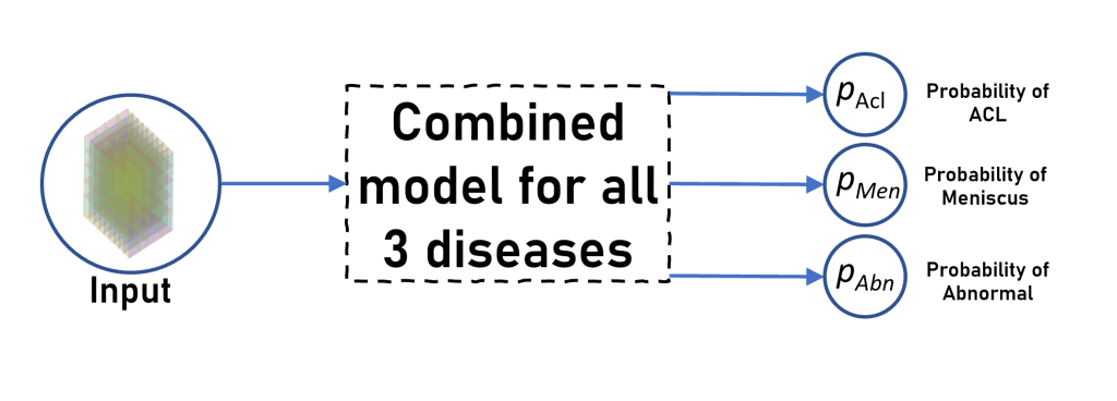
It should perform theoretically greater than or equal to the model for each disease that we trained above, since classifying one class might help the model to classify other classes as well since backpropogate the loss through all the classes.

So test the above claim, we made a single model for all 3 diseases and we will cover this in our next post along with the results

Conclusion

Congratulations on making this far, we know it was a lot to take in, so we will just summarize everything for you guys.

We got to know about the MRNet Challenge Dataset and the task that we had to do in this challenge.
We discussed some differences that this dataset has with the other image classification datasets.
We then trained 3 different models to classify MRI scans for each disease.
We then discussed some possible alternative approaches.
However due to the unique dataset, it wasn’t possible to provide relatable visualizations.

Thank you so much for reading this!

Until next time